
What is Gaussian splatting?
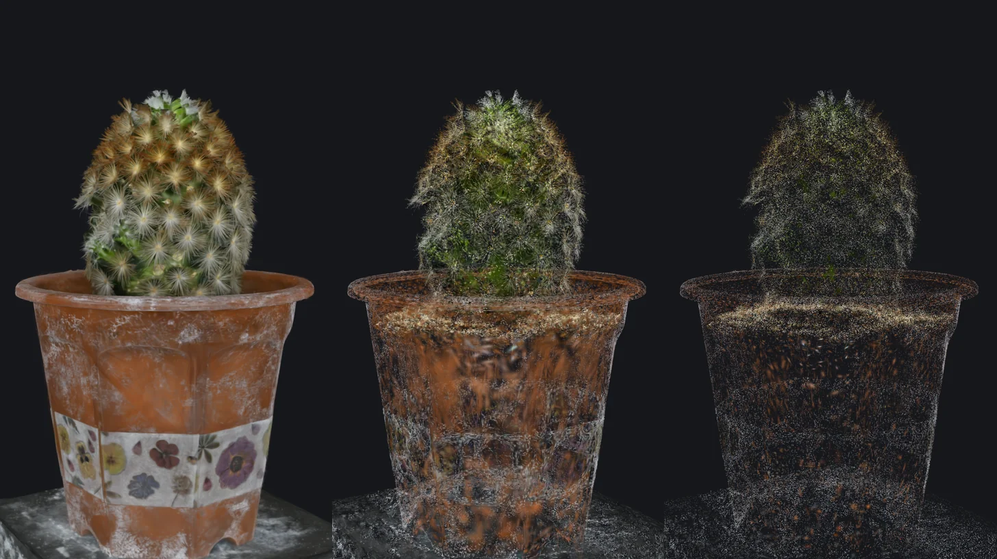
Gaussian splatting — or 3D Gaussian Splatting, often shortened to 3DGS — is a technique that represents a three-dimensional scene as hundreds of thousands, sometimes millions, of small soft blobs shaped like ellipsoids: Gaussians. Each one has a position, a shape, a color and a transparency; together they reproduce a photographed scene with near-photographic realism, and they render in real time.
The method was presented at SIGGRAPH 2023 by an Inria team: Bernhard Kerbl, Georgios Kopanas and George Drettakis, of the GRAPHDECO group at Inria and Université Côte d'Azur, with Thomas Leimkühler of the Max Planck Institute for Informatics. In three years it has gone from the lab to game engines, web browsers and an international standard.
The word splatting comes from splat: each Gaussian is projected onto the screen like a drop of paint, dense in the middle and fading towards the edges along a bell curve — the Gaussian curve that gives it its name.
A real scene, to turn around
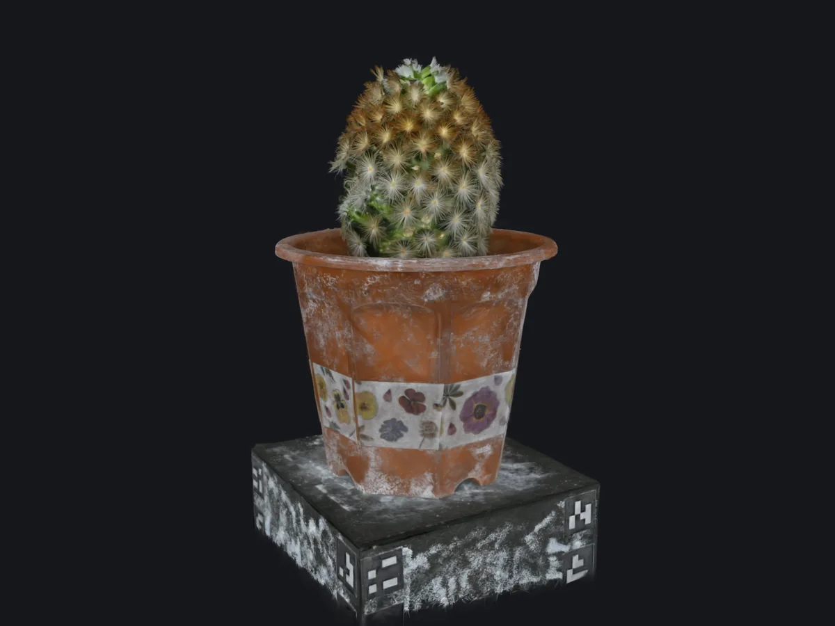
2.2 MB to download
Drag to turn · pinch, or Ctrl (⌘) + wheel, to zoom · keyboard: arrows, + and −
Scene: Steam Studio (steam-studio.jp), CC0 license — 427 photos, trained with Postshot.
A Gaussian splatting scene rendered live: a potted cactus on a stand, reconstructed from 427 photos. You can turn it, zoom, and shrink every splat until the scene comes apart into thousands of colored ellipses.
Turn the scene, then drag “Splat size” to the left: every Gaussian shrinks in place, and the object comes apart into thousands of colored blobs — the spines turn out to be long, very thin ellipses. Below about 10%, the splats become smaller than a pixel; the renderer then keeps them at a minimum size, as the reference method does, and they stay visible as dots. The “Opaque ellipsoids” mode draws every sufficiently opaque Gaussian as a solid shape, with no fade: the structure of the scene. To stay light, this view uses only each Gaussian’s base color (degree 0, explained below), without the highlights that change with the angle. The renderer was written for this article, in WebGL 2, without a library.
What is 3D Gaussian Splatting?
A Gaussian splatting scene has no surface and no triangles. It is a cloud of overlapping, semi-transparent Gaussians, drawn from back to front. Where they are dense and opaque you see an object; where they are sparse you see through. That absence of surface is exactly what lets it render what classic 3D meshes struggle with: foliage, hair, smoke, reflections, and very thin things like thorns or cables.
What is a Gaussian?
A 3D Gaussian is a soft, ellipsoid-shaped blob whose density falls off from the center to the edges. It is fully described by a handful of numbers:
- a position in space (3 numbers);
- a stretch along its three axes (3 numbers) and a rotation (4 numbers, as a quaternion) — together they form what researchers call the covariance, the blob's shape and orientation;
- an opacity (1 number);
- a color that changes with the viewing angle (48 numbers; more on that below).
That is 59 numbers per Gaussian. The scenes in the original paper hold between one and five million of them.
One Gaussian, by hand
Cross-section along the first axis: Gauss’s bell curve
Drag the handles. With the keyboard: arrow keys to adjust, Shift to move ten times faster.
A soft elliptical blob you can move, stretch in two directions, rotate and make more or less opaque. Underneath, its cross-section along the first axis: a bell curve.
Drag the handles or use the sliders. The curve underneath is a cross-section of the blob along its first axis: the bell curve that gives the method its name. In 3D there is a third axis, but the principle is the same.
Why blobs rather than triangles?
For decades, computer graphics has been built on triangles: a surface is cut into facets, and each facet is colored. It is remarkably efficient for objects with clean edges, but it assumes exact geometry, and anything without a well-defined surface — hair, a cloud, a dirty window — becomes a headache.
A Gaussian does not claim to describe a surface. It only says: "there is a bit of this color, roughly here". Because it is soft, two neighboring Gaussians blend into each other without a seam; because it can stretch and rotate, one elongated Gaussian is enough to draw a strand, an edge or a thorn. Above all, a soft blob changes smoothly: we can compute how the image changes when it moves a tiny amount, which means it can be adjusted automatically. That is the whole point of the method, as training will show.
Same budget, three building blocks
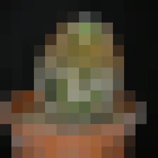
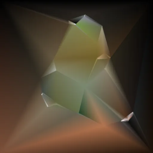
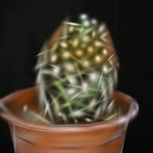
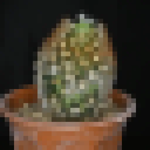
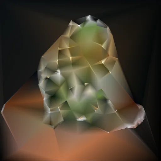
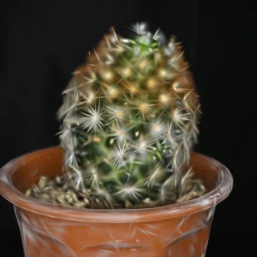
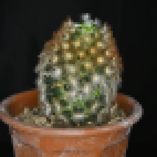
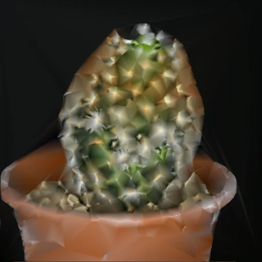
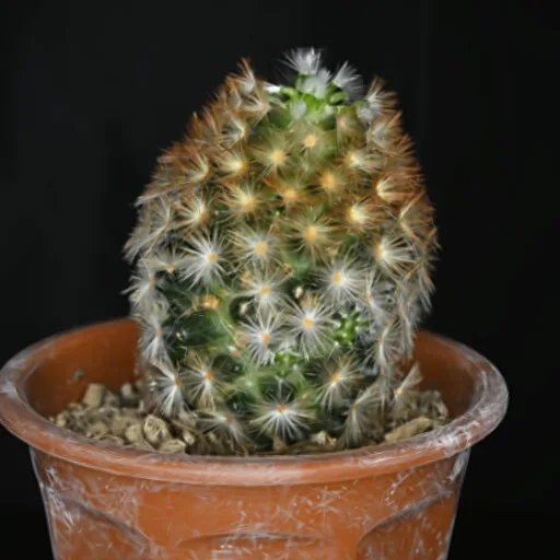
The same photo rebuilt with the same number of primitives: square pixels, shaded triangles, Gaussians. Pick the budget; under each image, its measured quality (PSNR) and how many values it stores.
For the same count, Gaussians keep the most of the photo, because each one can stretch, rotate and blend into its neighbors. But the same count is not the same size: a pixel stores 3 values (its color), a triangle vertex 5 (its position and color, shared by neighboring triangles), a 2D Gaussian 9 (position, two stretches, rotation, color, opacity). Even with the same number of values, Gaussians keep the lead: 200 Gaussians (1,800 values) beat 1,024 pixels (3,072 values). The triangles are placed by Garland and Heckbert’s greedy algorithm, which adds the worst-rendered point at each round, with vertex colors fitted as well as possible; the Gaussians come from the same fit as the training figure further down. PSNR: higher is better.
Where the color comes from
Of a Gaussian's 59 numbers, 48 are for its color. It is not a fixed color but a function of the direction you look from, encoded with spherical harmonics — a compact way to describe a value that varies all around a sphere. The same Gaussian can look bright head-on and dark from an angle.
This is what reproduces reflections and highlights. One distinction matters: a single Gaussian shows only one color at a time, which changes with the angle. A highlight sliding across a surface emerges from thousands of neighboring Gaussians, each changing color in its own way.
A color that depends on the angle
A single Gaussian shows a single color at a time: the one for the direction it is seen from.
- Outer ring: the true color seen from each direction
- Inner ring: what the Gaussian keeps of it
The highlight exists only as the agreement of several neighboring Gaussians.
Left, one Gaussian and a ring of every direction it can be seen from: the outer ring shows the color a shiny surface would have, the inner ring what the Gaussian can keep of it at the chosen degree. Right, sixteen Gaussians along a lit, curved surface: as the camera moves, the highlight slides from one to the next. At degree 0 the color no longer depends on the angle and the highlight disappears.
Drag on the drawings or use the sliders, then change the degree. At degree 0, 3 numbers are enough, but the color is the same from everywhere: no highlight. At degree 3, the one the reference method uses, 48 numbers draw a sharp highlight — with slight ripples around it, the limit of what 16 functions per channel can represent. A 2D figure: viewing directions are taken in a plane.
Comparison with other approaches
Photogrammetry
Photogrammetry is the long-standing way to digitize an object or a place from photos. You recover where each camera was, compute a point cloud, and derive a textured triangle mesh from it. The result is a real surface: measurable, and usable in every 3D tool.
Its weaknesses are well known. Anything without a clean surface (sky, foliage, hair), anything very thin (cables, fences, thorns), anything that reflects or lets light through (glass, water, polished metal) comes out holed, melted or warped.
Photogrammetry and Gaussian splatting are often set against each other. That is partly a false debate: both start from the same step, recovering the camera positions and a point cloud from the photos. What differs is what gets built next — a surface in one case, a cloud of Gaussians in the other. The splat wins on visual realism; the mesh stays more usable, since you can measure it, edit it and 3D-print it.
Same photos, two reconstructions
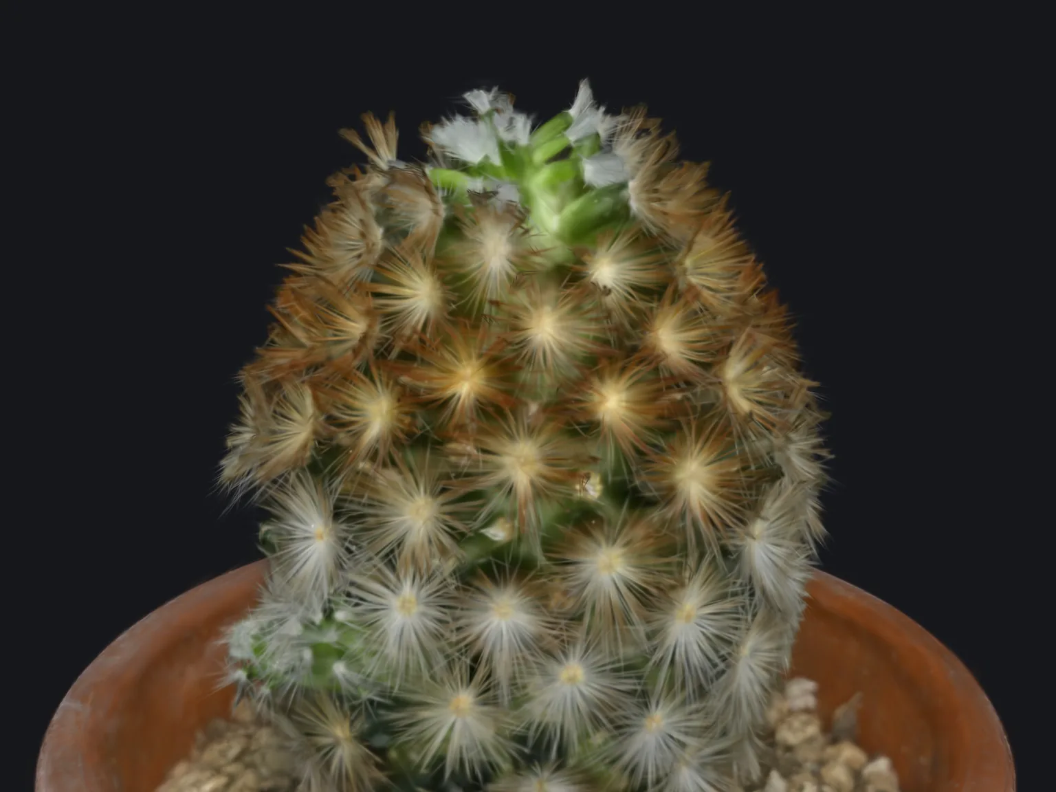
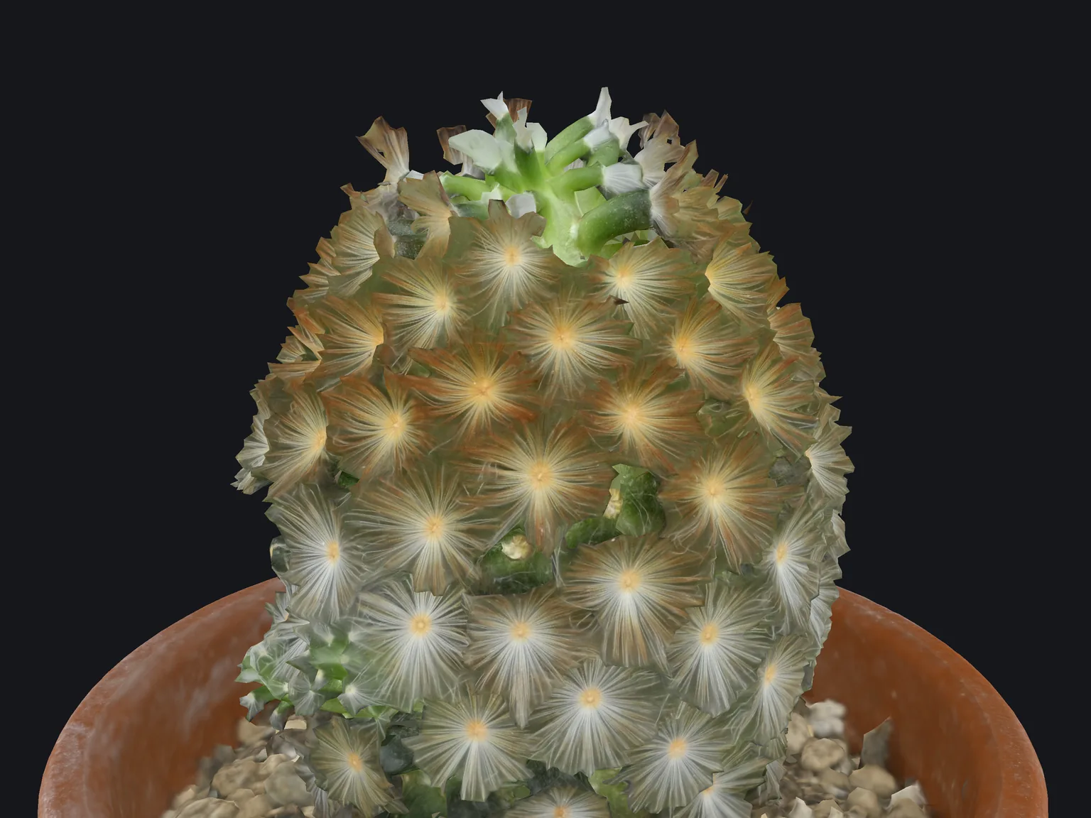
What to look for
- Face on, the mesh’s spines look sharp: they are painted into an 8,192-pixel texture on a smooth surface — like a photo stuck on a balloon. The splat, a little softer, draws them one by one, in relief, with their translucency.
- At the outline the illusion breaks: the mesh cuts the cactus into facets, like folded paper, and loses the tips of the spines; the splat keeps the spines that stick out — the plant’s real silhouette.
- The rim of the pot: the two line up to the pixel, because they come from the same photos and the same camera positions.
Data: Steam Studio (steam-studio.jp), CC0 license — 100,000-triangle RealityCapture mesh, 139,000-Gaussian Postshot splat.
The same cactus rebuilt from the same 427 photos: left as a textured mesh (photogrammetry), right as a Gaussian splat, seen from exactly the same viewpoint. A slider moves the split between the two.
Drag the split. The mesh has 100,000 triangles and an 8,192 × 8,192-pixel texture; the splat, 139,000 Gaussians. Neither is “better”: the mesh is a real surface that you can measure, edit or print; the splat renders better whatever has no clean surface. For this comparison we registered the mesh onto the splat, then rendered both images with the same camera.
NeRF
In 2020, Neural Radiance Fields (NeRF) showed that a neural network could learn a scene from photos and render new views of it with unprecedented realism, reflections included. The scene is implicit: to know the color at a point, you query the network. To draw a single image, you query it millions of times, along the ray of every pixel. Hence remarkable quality, but slow rendering and long training.
Gaussian splatting keeps the idea of learning the scene from photos, but replaces the network with an explicit set of Gaussians that can be drawn directly, the way triangles are drawn. That is what makes it so fast.
What the original paper's numbers say
The 2023 paper compares methods on the Mip-NeRF360 dataset, real scenes photographed in 360°. The best NeRF of the time, Mip-NeRF360, kept a slight edge on one of the three quality measures (27.69 dB of PSNR against 27.21) and was behind on the other two. But it needed 48 hours of training and rendered at 0.06 frames per second. Gaussian splatting reached comparable quality in 41 minutes and rendered at 134 frames per second — more than 2,000 times faster.
What the original paper measured
Frames per second (log scale) · higher is better
- Plenoxels 6.79
- Instant-NGP (base) 11.7
- Instant-NGP (big) 9.43
- Mip-NeRF360 † 0.06
- Gaussian splatting (7,000 it.) 160
- Gaussian splatting (30,000 it.) 134
Training time (log scale) · lower is better
- Plenoxels 25 min 49 s
- Instant-NGP (base) 5 min 37 s
- Instant-NGP (big) 7 min 30 s
- Mip-NeRF360 † 48 h
- Gaussian splatting (7,000 it.) 6 min 25 s
- Gaussian splatting (30,000 it.) 41 min 33 s
PSNR in decibels (axis cut to 22–28 dB) · higher is better
- Plenoxels 23.08
- Instant-NGP (base) 25.30
- Instant-NGP (big) 25.59
- Mip-NeRF360 † 27.69
- Gaussian splatting (7,000 it.) 25.60
- Gaussian splatting (30,000 it.) 27.21
Show the full table
| Method | PSNR (dB) | SSIM | Training | Frames/s | Memory |
|---|---|---|---|---|---|
| Plenoxels | 23.08 | 0.626 | 25 min 49 s | 6.79 | 2.1 GB |
| Instant-NGP (base) | 25.30 | 0.671 | 5 min 37 s | 11.7 | 13 MB |
| Instant-NGP (big) | 25.59 | 0.699 | 7 min 30 s | 9.43 | 48 MB |
| Mip-NeRF360 † | 27.69 | 0.792 | 48 h | 0.06 | 8.6 MB |
| Gaussian splatting (7,000 it.) | 25.60 | 0.770 | 6 min 25 s | 160 | 523 MB |
| Gaussian splatting (30,000 it.) | 27.21 | 0.815 | 41 min 33 s | 134 | 734 MB |
Source: Kerbl et al., 2023, Table 1, measured on an RTX A6000. † Quality figures the authors took from the Mip-NeRF360 paper.
Six methods compared on the Mip-NeRF360 dataset: rendering speed, training time and image quality, from Table 1 of the 2023 paper.
Speed and training time use logarithmic scales: without them, every method but one would be squashed against zero. The price of that speed is memory — 734 MB per scene for Gaussian splatting, against 8.6 MB for Mip-NeRF360.
How it works in detail
Structure from motion
It all starts with photos of the scene, taken from many angles. A structure from motion tool — historically COLMAP — finds points the photos have in common, works out the position and orientation of every shot, and reconstructs a sparse point cloud along the way. This step is classical geometry, not machine learning, and it is often the slowest and most fragile: from a few minutes to several hours depending on the number of photos, and sometimes an outright failure if the scene lacks texture or the photos overlap poorly.
This step is changing. Models such as VGGT, best paper at CVPR 2025, now estimate cameras and geometry in under a second, and are replacing COLMAP in a growing number of tools.
From points to Gaussians
Each point in the cloud becomes a Gaussian. Its position and color are known; its size is set from the distance to its nearest neighbors; its starting opacity is low. At this stage the scene is only a rough sketch. Everything that follows refines it.
Training: painting by trial and error
Training works like a painter correcting a canvas by constantly comparing it with the model. At each iteration, you take one of the photos, draw the Gaussians from the same viewpoint, and measure the difference between the result and the photo. Then every parameter of every Gaussian — position, shape, opacity, color — is nudged in the direction that reduces that difference.
It is gradient descent, as with a neural network, but without a network: the Gaussians themselves are what gets optimized. The difference combines a pixel-by-pixel error (weighted 80%) and a structural similarity measure (20%). The reference method runs 30,000 iterations, about forty minutes on a professional graphics card.
Training, one iteration at a time
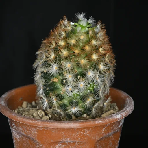
The photo
The Gaussians
Loading the training…
Iteration 6,000 · 1,600 Gaussians · PSNR 31.4 dB
Photo: Steam Studio (steam-studio.jp), CC0 license.
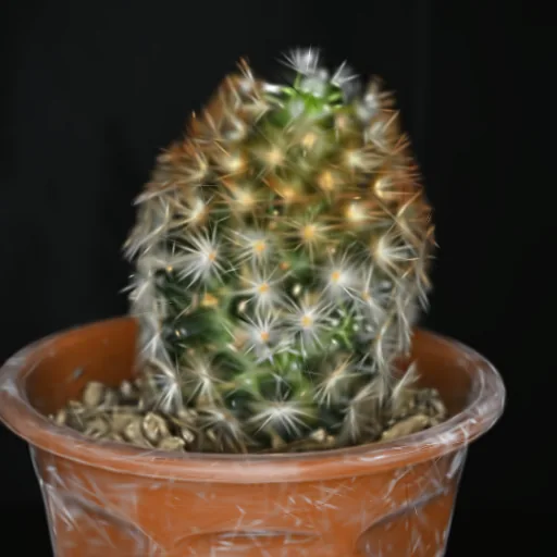
Left, a photo of a cactus. Right, the same photo repainted by two-dimensional Gaussians with the Gaussian splatting training loop: 256 blobs placed at random are compared with the photo, corrected, cloned, split and pruned, iteration after iteration. Two curves follow the image quality and the number of Gaussians.
Scrub through the iterations or press play. At the start, 256 blobs placed at random; within a few dozen iterations the colors settle. Densification then clones and splits Gaussians where the error stays high — the spines, the rim of the pot — up to the cap, set here at 1,600. At iteration 1,500 every Gaussian’s opacity is brought back close to zero: the image fades, then rebuilds itself within a few hundred iterations. The reference method does this every 3,000 iterations, to purge useless blobs. The “Error against the photo” display shows where the image still differs from the target: that is where the optimization pushes. The rules are the reference method’s, carried over to 2D (the thresholds are expressed as fractions of the image); the fit was computed in advance, and what you see is its replay.
Densification: clone, split, prune
The starting points are never enough. Some areas lack Gaussians; others have a single, oversized one where detail is needed. So every 100 iterations the method tidies up, guided by one simple signal: the size of the gradient, that is, how hard the optimizer is trying to move a Gaussian.
Densification: clone, split, prune
-
Step 1 · Diagnosis
Where the picture is wrong
Three cases. A small Gaussian (blue) borders a gap: the optimizer pulls it hard towards the empty area, and its gradient exceeds the 0.0002 threshold. A large, blurry Gaussian (amber) covers a detail it cannot render on its own. A third one (teal) is almost transparent and contributes nothing.
-
Step 2 · Clone
Small and in the wrong place: copy it
A small Gaussian with a high gradient is duplicated, and the copy is moved along the gradient, into the under-reconstructed area.
-
Step 3 · Split
Large and blurry: cut it in two
A large Gaussian with a high gradient is replaced by two Gaussians placed at random inside the old one, with their size divided by 1.6.
-
Step 4 · Prune
Almost transparent: remove it
A Gaussian whose opacity falls below 0.005 no longer contributes to the image. It is deleted.
-
Step 5 · Reset
Every 3,000 iterations, doubt everything again
Every Gaussian’s opacity is pushed back close to zero. The optimizer raises the ones that matter; those that stay transparent get pruned in turn.
The detail to reproduce
Five steps showing how the method adds Gaussians where detail is missing and removes the ones that do nothing.
The rules and thresholds are the reference method's; the positions are illustrative.
This mechanism multiplies the number of Gaussians as training goes on, up to several million for a full scene, while getting rid of the ones that do nothing.
Differentiable Gaussian rasterization
To show the scene, those millions of ellipsoids have to become pixels, on every frame. The process has three steps:
- Project each Gaussian onto the screen: a 3D ellipsoid becomes a soft 2D ellipse whose shape depends on the viewing angle and distance.
- Sort the Gaussians from nearest to farthest. The screen is cut into 16 × 16 pixel tiles, and sorting happens tile by tile, in parallel on the graphics card.
- Blend each pixel from front to back: each Gaussian adds its color in proportion to its opacity and to the light that is left, until the pixel is "full".
Sort, then blend
What the camera sees, reduced to one row of pixels
For this pixel: each Gaussian’s share of the color, then the light that is left
With sorting: the Gaussians are blended from nearest to farthest.
A top-down view of five Gaussians lettered A to E and a camera you can move around them. Below, the camera’s image, reduced to one row of pixels, then how much color each Gaussian adds to a chosen pixel.
A world reduced to two dimensions and seen from above, so everything fits in one figure: the camera's image is just one row of pixels. The projection, sorting and blending, however, are the real Gaussian splatting computations.
This rendering is called differentiable: for each pixel, we can compute how it would change if a given Gaussian moved. That is precisely what makes training possible — the same engine both displays the scene and learns it.
What has changed since 2023
The original paper described a promising but demanding technique: frozen scenes, files of several hundred megabytes, a dedicated graphics card, and a format almost nothing could read. Three years later, nearly every one of those limits has been lifted.
Three years of Gaussian splatting
-
The Inria team presents 3D Gaussian Splatting at SIGGRAPH: NeRF-level quality, rendered at 134 frames per second.
-
4DGS adds time to the Gaussians and renders dynamic scenes at 82 frames per second.
-
pixelSplat predicts Gaussians directly from two images, with no per-scene training.
-
Scaniverse trains splats directly on the phone.
-
Niantic open-sources the SPZ format: 64 bytes per Gaussian instead of 236.
-
VGGT estimates cameras and geometry in under a second and starts replacing COLMAP.
-
NVIDIA’s 3DGUT, now in the gsplat library, handles fisheye lenses and secondary rays.
-
World Labs opens Marble to everyone: worlds created from text or an image, exportable as splats.
-
OpenUSD 26.03 adds a native schema for Gaussian splats.
-
A hundred million in a browser
Spark 2.0 streams worlds of more than 100 million Gaussians on the web.
-
The KHR_gaussian_splatting extension is ratified by the Khronos Group.
The milestones between the method’s publication in 2023 and its standardization in 2026, each linked to its source.
Each milestone links to its primary source.
Scenes that move
As early as autumn 2023, so-called "4D" variants added time: Gaussians that move and deform from frame to frame. 4DGS already rendered dynamic scenes at 82 frames per second. In 2026 these animated splats are used to stream volumetric video — a music performance filmed in 4D splats was streamed this spring, watchable in a browser as well as in a headset.
Files ten times lighter
A scene in the original paper weighed 734 MB on average. Compressed formats changed that. SPZ, open-sourced by Niantic in 2024, takes a Gaussian from 236 bytes to 64. SOG, PlayCanvas's open format, fits a 4-million-Gaussian scene into 42 MB instead of roughly 1 GB.
A standard format
In early September 2026, the glTF extension KHR_gaussian_splatting reached "ratified" status with the Khronos Group, the body behind glTF, often called "the JPEG of 3D". Cesium, Niantic, Esri, NVIDIA and Autodesk are among its contributors. OpenUSD, the scene description format that started at Pixar, added a native schema for splats in March 2026. One caveat: compression is not part of the ratified extension; it is handled by separate extensions that are still drafts.
No training needed
Per-scene training is no longer the only route. Some models predict the Gaussians directly from a few photos in a fraction of a second: pixelSplat from two images as early as 2023, AnySplat in 2025 from photos with unknown positions, or Apple's SHARP from a single image. Further still, generative "world" models such as Marble or World Labs' Atlas produce whole scenes that export as splats, with no capture at all.
On a phone, in a browser
In 2023 the reference viewer called for a dedicated graphics card. In 2026 a phone is enough. On an iPhone 13 Pro Max, in a browser, PlayCanvas's WebGPU engine renders 4 million Gaussians at 42 frames per second (at 642 × 1126 pixels). Spark 2.0 streams worlds of more than 100 million Gaussians, and visionOS 27 renders them natively on Apple's headset. One more caveat: on Meta's Quest headset, Hyperscape renders on Meta's servers and streams the result. That is not on-device rendering.
Advantages and disadvantages in 2026
Advantages
- Realism: near-photographic rendering, including foliage, hair, reflections and thin objects.
- Speed: real-time display, down to a phone in a browser.
- Accessible capture: for many subjects, a few minutes of smartphone video are enough.
- A mature ecosystem: compressed formats, a ratified glTF standard, support in the main 3D tools.
Disadvantages
- No usable surface: a splat is hard to measure and hard to edit, and turning it into a mesh takes dedicated methods.
- No metric guarantee: scale and accuracy depend entirely on the capture. That is the subject of our article on what an iPhone, 360 camera or LiDAR capture guarantees.
- Baked lighting: the light is "baked" into the colors. Relighting a scene is still a research problem.
- Artifacts: floating Gaussians (floaters) in poorly photographed areas, and blur as soon as you stray too far from the capture viewpoints.
- Raw weight: uncompressed, a large scene still easily exceeds a gigabyte.
You often read that it takes "12 GB of graphics memory" or "1 GB per scene". The original paper's figures are different: 734 MB per scene on average, and a peak above 20 GB during training with the research code. Both have shrunk since, thanks to compressed formats and optimized implementations.
Creating and viewing a Gaussian splat
To capture a scene, a smartphone is often enough: walk slowly around the subject, filming or photographing, with plenty of overlap between views. Apps like Scaniverse even train the splat on the phone itself; Polycam does it in the cloud. For finer control, tools such as Postshot, LichtFeld Studio or Brush train on a computer, and SuperSplat lets you clean up and edit the result in a browser. For a fuller survey of the tools, see our article on the Gaussian splatting ecosystem. Each stage — capture, camera poses, training, cleaning, compression, publishing — is detailed, with measured file sizes, in the Gaussian splatting production workflow.
As for formats, PLY remains the universal raw output; SPZ and SOG are the most widespread compressed formats; and glTF, with the KHR_gaussian_splatting extension, is becoming the standard exchange format.
This is where our own work begins. Everything ARGO builds runs in the browser, with no app to install — and a well-compressed splat now suits that perfectly: it opens on the visitor's phone from a QR code or a link, with the realism of a photograph and the freedom of movement of 3D.
FAQ
Frequently asked questions
Sources and further reading
- Kerbl, Kopanas, Leimkühler, Drettakis, 3D Gaussian Splatting for Real-Time Radiance Field Rendering, ACM Transactions on Graphics 42(4), SIGGRAPH 2023 — arXiv:2308.04079 · project page, Inria
- Dylan Ebert, Introduction to 3D Gaussian Splatting, Hugging Face, 2023 — huggingface.co
- Aras Pranckevičius, Gaussian Splatting is pretty cool!, 2023 — aras-p.info
- Three surveys of the research: Chen and Wang, arXiv:2401.03890 · Fei et al., arXiv:2402.07181 · Wu et al., arXiv:2403.11134
- Khronos Group, KHR_gaussian_splatting specification
- Niantic, SPZ format · PlayCanvas, SOG format and WebGPU mobile benchmarks · World Labs, Spark 2.0
Figures and statuses checked in September 2026.